Huffman, Arithmetic Coding, and ANS: Data Compression Techniques

Introduction
Data compression is a crucial field in computer science, providing the means to store and transmit data efficiently. As digital data continues to grow exponentially, the importance of effective compression techniques cannot be overstated. Compression algorithms reduce the amount of data needed to represent a file or message, enabling faster data transmission and saving storage space. In this guide, we will delve deep into three essential data compression algorithms:
- Huffman Coding: A widely-used algorithm that assigns variable-length codes to input characters, optimizing the encoding based on character frequency.
- Arithmetic Coding: A more advanced technique that represents entire messages as fractions within a specific range, allowing for more efficient compression.
- Asymmetric Numeral Systems (ANS): A modern and innovative approach that combines the strengths of arithmetic coding with faster performance by using natural numbers and dynamic labeling.
This guide will provide an in-depth understanding of each algorithm, its mechanics, advantages, and limitations, supported by detailed examples, diagrams, and practical applications.
1. Huffman Coding: The Foundation of Data Compression
1.1 Overview of Huffman Coding
Huffman coding, developed by David A. Huffman in 1952, is one of the simplest and most widely used data compression algorithms. It belongs to the family of lossless data compression algorithms, which means that the original data can be perfectly reconstructed from the compressed data. Huffman coding assigns variable-length codes to input characters, with shorter codes assigned to more frequent characters. This results in a compressed output that minimizes the overall bit-length of the encoded data.
1.2 How Huffman Coding Works
Step 1: Frequency Analysis
- Analyze the input data to determine the frequency of each character.
- Example: Consider the text "ABBCCCDDDDEEEEE":
- A: 1, B: 2, C: 3, D: 4, E: 5.
Step 2: Building the Huffman Tree
- Create a priority queue (or a binary tree) where each node is a character with its frequency.
- Combine the two nodes with the lowest frequencies to create a new node with a combined frequency. Repeat this process until only one node remains, forming the root of the tree.
Step 3: Generating Huffman Codes
- Traverse the Huffman tree from the root to each leaf node. Assign a '0' for left branches and a '1' for right branches.
- The path to each character determines its binary code.
1.3 Example of Huffman Coding
Using the string "ABBCCCDDDDEEEEE" across all examples ensures consistency:
- Frequency Table:
| Character | Frequency |
|---|---|
| A | 1 |
| B | 2 |
| C | 3 |
| D | 4 |
| E | 5 |
Building the Huffman Tree:
- Combine A (1) and B (2) to form a node with frequency 3.
- Combine this node (3) with C (3) to form a node with frequency 6.
- Combine this node (6) with D (4) to form a node with frequency 10.
- Combine this node (10) with E (5) to form the root node with frequency 15.
Huffman Tree Diagram:
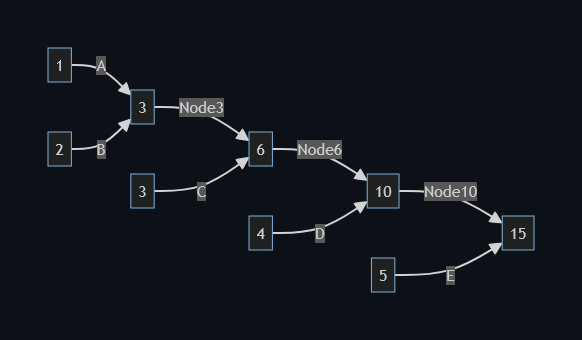
- Generating Huffman Codes:
- A: 1100
- B: 1101
- C: 111
- D: 10
- E: 0
The encoded message "ABBCCCDDDDEEEEE" using Huffman coding is:
1100 1101 1101 111 111 111 10 10 10 10 0 0 0 0 0
1.4 Advantages and Limitations of Huffman Coding
Advantages:
- Simple to understand and implement.
- Effective for data with a clear variance in character frequency.
- Guaranteed to produce an optimal prefix code for the given symbol frequencies.
Limitations:
- Not suitable for data where symbol frequencies are nearly uniform.
- Requires knowledge of symbol frequencies beforehand, which may not always be available or feasible.
- Inefficient for small datasets or real-time applications due to tree-building overhead.
1.5 Complexity of Huffman Coding
- Time Complexity: Building the Huffman tree has a time complexity of (O(n \log n)), where (n) is the number of unique characters. This is due to the sorting and merging operations involved in constructing the tree.
- Space Complexity: The space complexity is (O(n)) for storing the tree and the frequency table.
1.6 Practical Applications of Huffman Coding
Huffman coding is widely used in various data compression applications:
- Image Compression: JPEG and PNG file formats utilize Huffman coding for lossless compression of image data.
- Text Compression: Frequently used in file compression utilities like ZIP.
- Data Transmission: Helps reduce the size of data packets for efficient network transmission.
1.7 Historical Context and Future Directions
Huffman coding has been a foundational algorithm in the field of data compression since its introduction. Its simplicity and effectiveness have made it a staple in many early compression systems. However, as data and computing needs evolve, Huffman coding faces limitations in efficiency, especially with real-time data and larger datasets. Future advancements may focus on hybrid models that combine Huffman coding with more sophisticated techniques to improve efficiency and adaptability.
2. Arithmetic Coding: Precision in Compression
2.1 Overview of Arithmetic Coding
Arithmetic coding is a sophisticated data compression technique that goes beyond the limitations of Huffman coding. Instead of assigning fixed codes to individual symbols, arithmetic coding represents the entire message as a single fractional value between 0 and 1. This allows it to achieve higher compression ratios, especially for data with skewed probability distributions.
2.2 How Arithmetic Coding Works
Step 1: Initial Range Setting
- Begin with the entire range [0, 1).
Step 2: Subdividing the Range
- For each symbol, subdivide the current range into smaller segments proportional to the symbol's probability.
Step 3: Narrowing Down the Range
- As each symbol is processed, the range is narrowed to represent the message uniquely.
2.3 Example of Arithmetic Coding
Using the same string "ABBCCCDDDDEEEEE" ensures consistency:
Assume simplified symbol probabilities for the demonstration:
| Symbol | Probability |
|---|---|
| A | 0.1 |
| B | 0.2 |
| C | 0.2 |
| D | 0.2 |
| E | 0.3 |
Encoding Process:
Start with the range [0, 1).
Encoding A:
- Range is subdivided into:
- A: [0, 0.1), B: [0.1, 0.3), C: [0.3, 0.5), D: [0.5, 0.7), E: [0.7, 1).
- After encoding
A, the range is [0, 0.1).
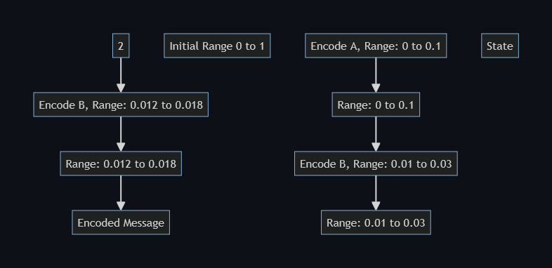
Encoding B within [0, 0.1):
- Subdivide range into:
- A: [0, 0.01), B: [0.01, 0.03), C: [0.03, 0.05), D: [0.05, 0.07), E: [0.07, 0.1).
- After encoding
B, the range is [0.01, 0.03).
Encoding another B within [0.01, 0.03):
- Subdivide range into:
- A: [0.01, 0.012), B: [0.012, 0.018), C: [0.018, 0.024), D: [0.024, 0.026), E: [0.026, 0.03).
- After encoding another
B, the range is [0.012, 0.018).
The encoded message "ABB" can be represented by any number in the range [0.012, 0.018), such as 0.015.
2.4 Visualization of Arithmetic Coding
Below is a visual representation of the arithmetic coding process, illustrating how the range is subdivided for each symbol.
2.5 Pros and Cons of Arithmetic Coding
Advantages:
- Can handle any probability distribution, achieving optimal compression.
- More efficient than Huffman coding, especially for data with complex symbol distributions.
- Produces near-optimal entropy coding.
Disadvantages:
- Computationally intensive, requiring more processing power than Huffman coding.
- Historically faced patent-related adoption barriers.
- More challenging to implement, requiring precision in handling fractional numbers.
2.6 Complexity of Arithmetic Coding
- Time Complexity: Arithmetic coding has a time complexity of (O(n)), where (n) is the length of the input data. Each symbol requires constant time to process.
- Space Complexity: The space complexity is also (O(n)) due to the need to store the input, output, and range values for each symbol.
2.7 Practical Applications of Arithmetic Coding
Arithmetic coding is used in applications where high compression ratios are essential:
- Multimedia File Formats: Video codecs like H.264 and H.265 use arithmetic coding for entropy encoding.
- Data Compression: Commonly used in text compression and data archival systems where maximum efficiency is required.
- Embedded Systems: Finds use in systems where memory and storage are at a premium.
2.8 Historical Context and Future Directions
Introduced in the 1970s, arithmetic coding has been critical in advancing data compression. Its ability to handle complex distributions made it superior to Huffman coding in many applications. The primary barriers to its adoption were patent restrictions, which have since expired, allowing more widespread use. Future directions may involve optimizing arithmetic coding for faster computation and adapting it to modern real-time processing needs.
3. Asymmetric Numeral Systems (ANS): A New Frontier in Compression
3.1 Introduction to Asymmetric Numeral Systems
Asymmetric Numeral Systems (ANS) is a relatively new compression algorithm that combines the efficiency of arithmetic coding with the speed and simplicity of table-based methods. ANS uses a clever approach by encoding data as natural numbers, making it well-suited for real-time applications. It provides a high compression rate while being computationally less demanding than traditional arithmetic coding.
3.2 How ANS Works
Step 1: Labeling Natural Numbers
- ANS starts by labeling natural numbers based on symbol frequencies. Each number is labeled with a symbol, ensuring that the frequency of each symbol matches its probability.
Step 2: Encoding a Message
- Each symbol is encoded by transforming the current state into a new state using a predefined function. The transformation depends on the symbol being encoded and the current state.
Step 3: Renormalization
- When the state becomes too large, it is renormalized to maintain the encoding efficiency. This process involves shifting bits out and maintaining a manageable state size.
3.3 Example of ANS Encoding
Using the same string "ABBCCCDDDDEEEEE" ensures consistency:
Assume simplified symbol probabilities:
| Symbol | Probability |
|---|---|
| A | 0.1 |
| B | 0.2 |
| C | 0.2 |
| D | 0.2 |
| E | 0.3 |
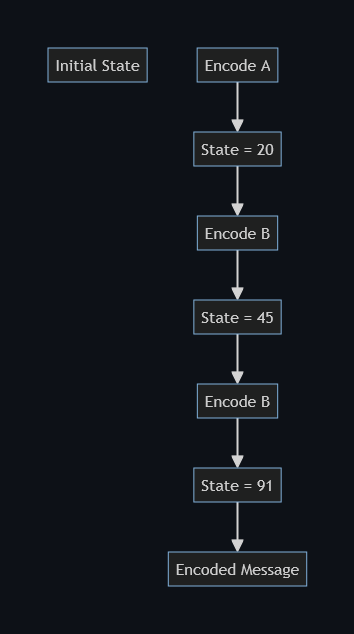
- Initial State: Choose an initial state, e.g., (X = 10).
- Encoding
A:
- Find the next state for
A, using a table-based approach or predefined function. The state may become (X = 20).
- Encoding
B:
- Update the state based on
B, such as (X = 45).
- Encoding another
B:
- Update the state again, e.g., (X = 91).
3.4 Visualization of ANS Encoding
Below is a conceptual diagram of the ANS encoding process, showing how natural numbers are labeled and how the state transitions during encoding.
3.5 Advantages and Limitations of ANS
Advantages:
- Combines the efficiency of arithmetic coding with the speed of table-based methods.
- Suitable for real-time applications due to its fast encoding and decoding processes.
- No floating-point arithmetic needed, reducing computational complexity.
- Public domain algorithm, avoiding the patent issues that hindered arithmetic coding.
Limitations:
- More complex to understand and implement than Huffman coding.
- Performance depends on the proper design of symbol labeling and state transitions.
- Limited ability to handle adaptive contexts compared to arithmetic coding.
3.6 Complexity of ANS
- Time Complexity: ANS offers a time complexity of (O(1)) per symbol due to its table-driven nature, making it extremely fast.
- Space Complexity: The space complexity is (O(n)), where (n) is the number of symbols, as it requires space to store tables and state information.
3.7 Practical Applications of ANS
ANS is rapidly gaining popularity in modern applications:
- JPEG XL: Uses ANS for efficient and fast image compression, aiming to replace older JPEG formats.
- Video Encoding: Incorporated into video codecs to improve compression rates and decoding speed.
- Real-Time Data Streaming: Ideal for scenarios requiring low-latency data transmission, such as live video streaming.
3.8 Historical Context and Future Directions
ANS, introduced by Jarek Duda in the early 2010s, represents a significant leap forward in compression technology. By addressing the speed limitations of arithmetic coding while maintaining efficiency, ANS has become a preferred choice for many real-time and high-performance applications. As research continues, we can expect further optimizations and potential adaptations of ANS to support adaptive contexts and other advancements.
Conclusion
Data compression is a vital tool in the digital age, enabling efficient storage and transmission of information. Understanding the principles and mechanisms behind different compression algorithms can significantly impact how we handle data. Here's a summary of the key points covered:
Summary
- Huffman Coding is a foundational technique in data compression, suitable for cases with variable symbol frequencies. It constructs a binary tree and assigns shorter codes to more frequent symbols.
- Arithmetic Coding offers higher compression rates by encoding entire messages as fractional numbers, providing near-optimal compression for complex data distributions. It faces challenges in implementation and computational efficiency.
- Asymmetric Numeral Systems (ANS) brings together the best of both worlds, achieving high compression efficiency with faster encoding and decoding speeds. It is becoming increasingly popular in applications that demand both high compression ratios and low latency.
Visual Summary
Here is a visual representation to highlight the differences between these three compression methods:
- Huffman Coding Tree: Visualizing how characters are represented by variable-length codes based on symbol frequency.
- Arithmetic Coding Flowchart: Illustrating the process of subdividing the range for each symbol to encode a message.
- ANS Encoding Diagram: Demonstrating the steps involved in encoding a message using ANS.
Further Reading and Resources
- Wikipedia: Huffman Coding
- Wikipedia: Arithmetic Coding
- Wikipedia: Asymmetric Numeral Systems
- David Salomon's "Data Compression: The Complete Reference"
- Jarek Duda's Research on ANS
By understanding these algorithms, you can select the most appropriate compression method for your specific needs, whether it be for image storage, video streaming, or efficient data transmission. As technology continues to advance, mastering these techniques will become increasingly crucial in managing the vast amounts of digital data generated daily.